Interpolation_Tutorial

Table of Contents

• Interpolation Tutorial
  • Introduction
  • Example - Inverse Distance Weighted (IDW) Interpolation
  • Example - Linear Interpolation
  • Example - Natural Neighbor Interpolation
  • Example - Anisotropic Interpolation

Interpolation Tutorial

Introduction

The purpose of this tutorial is to provide explanation on how to use the classes defined in xmsinterp to perform spatial interpolation. The examples provided in this tutorial refer to test cases that are in the xmsinterp/tutorial/TutInterpolation.cpp source file.

The xmsinterp library contains classes for performing 2d (x,y) linear, natural neighbor, and idw interpolation: xms::InterpLinear and xms::InterpIdw. Natural neighbor interpolation is performed using the linear interpolation class. 3d (x,y,z) interpolation can be performed using the idw class.

Both interpolators are derived off of xms::InterpBase. This class has methods for setting the points and triangles used to interpolate as well as methods to set scalar values and activity on points and triangles (you can imagine activity as points or cells that may have a “dry” value when the scalars are generated from a numerical model). At a minimum, you must specify the points to set up an interpolation class. The InterpLinear class requires triangles to perform the interpolation. If none are specified then the points are triangulated using xms::TrTriangulator;

Example - Inverse Distance Weighted (IDW) Interpolation

The following example shows how to use the IDW interpolator. The testing code for this example is TutInterpolationTests::test_Example_IDW.

void TutInterpolationIntermediateTests::test_Example_IDW()
{
  BSHP<xms::VecInt> tris(new xms::VecInt()); // not used by idw

  // Create the points used to interpolate
  BSHP<xms::VecPt3d> pts(new xms::VecPt3d());
  *pts = {{0, 0, 0}, {10, 0, 1}, {10, 10, 2}, {0, 10, 3}};

  // create the interpolator class
  BSHP<xms::InterpIdw> interp = xms::InterpIdw::New();
  // Set the points and triangles used by the interpolator. The triangles are
  // empty and are not used by idw.
  interp->SetPtsTris(pts, tris);

  // interpolate to a location
  xms::Pt3d loc(5, 5, 0);
  float val = interp->InterpToPt(loc);

  // verify the value
  float base(1.5);
  TS_ASSERT_EQUALS(base, val);

} // TutInterpolationIntermediateTests::test_Example_IDW

Example - Linear Interpolation

The following example shows how to use the Linear interpolator. The testing code for this example is TutInterpolationTests::test_Example_Linear.

void TutInterpolationIntermediateTests::test_Example_Linear()
{
  // Create the points used to interpolate
  BSHP<xms::VecPt3d> pts(new xms::VecPt3d());
  *pts = {{0, 0, 0}, {10, 0, 1}, {10, 10, 2}, {0, 10, 3}};

  // Create the triangles used to interpolate. The triangles are specified as
  // 3 indexes that refer to the points vector. The indexes should be ordered
  // counter clockwise.
  BSHP<xms::VecInt> tris(new xms::VecInt());
  *tris = {0, 1, 3, 1, 2, 3};

  // create the interpolator class
  BSHP<xms::InterpLinear> interp = xms::InterpLinear::New();
  // Set the points and triangles used by the interpolator.
  interp->SetPtsTris(pts, tris);

  // interpolate to a location
  xms::Pt3d loc(2, 1, 0);
  float val = interp->InterpToPt(loc);

  // verify the value
  float base(0.5);
  TS_ASSERT_EQUALS(base, val);
} // TutInterpolationIntermediateTests::test_Example_Linear

Example - Natural Neighbor Interpolation

The following example shows how to use the Natural Neighbor interpolator. This is an option that can be set on the xms::InterpLinear class. The testing code for this example is TutInterpolationTests::test_Example_NaturalNeighbor.

void TutInterpolationIntermediateTests::test_Example_NaturalNeighbor()
{
  // Create the points used to interpolate
  BSHP<xms::VecPt3d> pts(new xms::VecPt3d());
  *pts = {{0, 0, 0}, {10, 0, 1}, {10, 10, 2}, {0, 10, 3}};

  // Create the triangles used to interpolate. The triangles are specified as
  // 3 indexes that refer to the points vector. The indexes should be ordered
  // counter clockwise.
  BSHP<xms::VecInt> tris(new xms::VecInt());
  *tris = {0, 1, 3, 1, 2, 3};

  // create the interpolator class
  BSHP<xms::InterpLinear> interp = xms::InterpLinear::New();
  // Set the points and triangles used by the interpolator.
  interp->SetPtsTris(pts, tris);

  int nodalFunc = 0;            // 0 constant, 1 gradient plane, 3 quadratic
  int nodalFuncOpt = 1;         // 0 natural neighbors, 1 nearest n points
  int nNearest = 12;            // 12 nearest points used for nodal function
  bool blendWeights = false;    // flag to add weight blending
  BSHP<xms::Observer> progress; // observer to get feedback
  // set to use natural neighbor interpolation
  interp->SetUseNatNeigh(true, nodalFunc, nodalFuncOpt, nNearest, blendWeights, progress);

  // interpolate to a location
  xms::Pt3d loc(2, 1, 0);
  float val = interp->InterpToPt(loc);

  // verify the value
  float base(0.46f);
  TS_ASSERT_EQUALS(base, val);
} // TutInterpolationIntermediateTests::test_Example_NaturalNeighbor

Example - Anisotropic Interpolation

The following example shows how to use the Anisotropic Interpolator. The testing code for this example is TutInterpolationIntermediateTests::test_Example_Anisotropic.

void TutInterpolationIntermediateTests::test_Example_Anisotropic()
{
  // Create the centerline points.  The segments of this polyline will be mapped
  // onto the x-axis.  The total length will be preserved.
  xms::VecPt3d centerline = {{0, 0, 0}, {20, 0, 0}, {40, 20, 0}, {60, 20, 0}};

  // Create the points used to interpolate. These points are typically taken
  // from cross sections across the center line.  These points will be
  // transformed so that the x-coordinate corresponds to the intersection of a
  // line through the point and perpendicular to a segment of the centerline.
  // The y coordinate will be the distance above or below that intersection.
  // Note that a single point may project onto several segments, generating
  // multiple transformed points.
  xms::VecPt3d interpolationPoints = {
    // cross-section 1
    {0, 10, 100},
    {0, -10, 100},
    // cross-section 2
    {10, 10, 90},
    {10, 5, 60},
    {10, 0, 50},
    {10, -5, 70},
    {10, -10, 90},
    // cross-section 3
    {20, 20, 80},
    {30, 10, 40},
    {40, 0, 80},
    // cross-section 4
    {30, 40, 70},
    {35, 30, 50},
    {40, 20, 30},
    {45, 10, 70},
    // cross-section 5
    {60, 30, 50},
    {60, 10, 50},
  };

  // create the interpolator class
  BSHP<xms::InterpAnisotropic> interpolator = xms::InterpAnisotropic::New();

  // Set the centerline and interpolation points used by the interpolator.
  // Any point may project onto several segments of the centerline. You can use
  // all such transformed points or set pickClosest to true to use only the
  // one nearest the centerline.
  bool pickClosest = false;
  interpolator->SetPoints(centerline, interpolationPoints, pickClosest);

  // After the points are transformed, an inverse distance weighted
  // interpolation is done (using all of the interpolation points) after scaling
  // the points in the x direction.  The default x scale factor is 1.  Set to a
  // value less than 1 to compress the x values (thus giving them more weight
  // than y) or to a value greater than 1 (to have the opposite effect).
  interpolator->SetXScale(0.5);

  // Set the exponent of the inverse distance weight to a value over 1 to dilute
  // the influence of interpolation points far from the point in question.
  interpolator->SetPower(3);

  // You can access the actual transformed interpolation points as shown below.
  // This isn't necessary for the interpolation, but is useful if you want
  // plot and visualize the transformation.
  xms::VecPt3d snPoints;
  interpolator->GetInterpolationPts(snPoints);
  // clang-format off
  xms::VecPt3d expectedSnPoints = {
    // cross-section 1
    {0, 10, 100}, // 0
    {0, -10, 100}, // 1
    // cross-section 2
    {5, 10, 90}, // 2
    {10, 14.142, 90}, // 2
    {5, 5, 60}, // 3
    {5, 0, 50}, // 4
    {5, -5, 70}, // 5
    {5, -10, 90}, // 6
    // cross-section 3
    {10, 20, 80}, // 7
    {17.071, 14.142, 80}, // 7
    {17.071, 0, 40}, // 8
    {17.071, -14.142, 80}, // 9
    {24.142, -20, 80}, // 9
    // cross-section 4
    {24.142, 22.361, 70}, // 10
    {24.142, 11.180, 50}, // 11
    {24.142, 0, 30}, // 12
    {24.142, 0, 30}, // 12
    {22.374, -10.607, 70}, // 13
    {26.642, -10, 70}, // 13
    // cross-section 5
    {34.142, 10, 50}, // 14
    {34.142, -10, 50} // 15
  };
  TS_ASSERT_DELTA_VECPT3D(expectedSnPoints, snPoints, 0.01);
  // interpolate to a location and verify the value.
  xms::Pt3d loc(20, 5, 0);
  float val = interpolator->InterpToPt(loc);
  float base(59.5313f);
  TS_ASSERT_DELTA(base, val, 0.001);

  // interpolate to several locations and verify the values.  Note that the
  // last two points are beyond the range of the centerline; hence, they
  // generate no data (XM_NODATA) interpolation values.
  xms::VecPt3d interpToPoints = {
    {5, 5, 0},   {5, 0, 0},   {5, -5, 0},
    {20, 5, 0},
    {20, 0, 0},
    {20, -5, 0}, {10, 20, 0}, {30, -5, 0}, {30, 30, 0},
    {35, 20, 0}, {45, 25, 0}, {45, 15, 0},
    {65, 20, 0}, {-5, 0, 0}};

  // The transformed values of interpolated to points can be retrieved by
  // using GetTransformedPts. The transformed points could be used for
  // plotting or using another interpolation method.
  xms::VecPt3d snInterpToPoints;
  interpolator->GetTransformedPts(interpToPoints, false, snInterpToPoints);
  xms::VecPt3d expectedSnInterpToPoints = {
    {2.5, 5, 0}, {2.5, 0, 0},  {2.5, -5, 0}, // points 0, 1, 2
    {10, 5, 0},  {11.768, 3.536, 0},  // point 3 is transformed to 2 stations
    {10, 0, 0},  {10, 0, 0}, // point 4 is transformed to segment 0 { param 1 } and segment 1 { param 0 }
    {10, -5, 0}, {5, 20, 0}, {13.536, 21.213, 0}, {11.768, -10.607, 0}, // points 5, 6, 7
    {24.142, 14.142, 0}, {22.374, 3.536, 0}, {26.642, 5, 0}, // points 8, 9, 10
    {24.142, -7.071, 0},  {26.642, -5, 0}}; // point 11 is transformed to 2 stations
  // clang-format on
  TS_ASSERT_DELTA_VECPT3D(expectedSnInterpToPoints, snInterpToPoints, 0.001);

  xms::VecFlt interpValues;
  interpolator->InterpToPts(interpToPoints, interpValues);
  xms::VecFlt expectedInterpValues = {64.614f,  54.390f, 71.970f,          59.531f,         58.468f,
                                      68.0917f, 81.688f, 76.032f,          53.130f,         35.413f,
                                      40.457f,  50.839f, (float)XM_NODATA, (float)XM_NODATA};
  TS_ASSERT_DELTA_VEC(expectedInterpValues, interpValues, 0.01);

} // TutInterpolationIntermediateTests::test_Example_Anisotropic

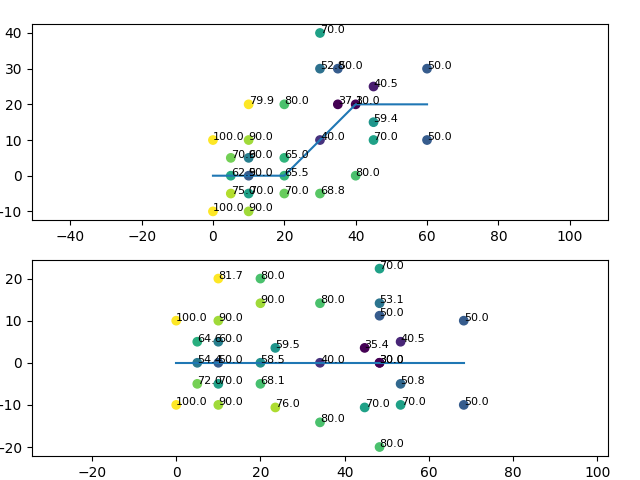
The data for this example is shown in the plot below. The upper figure shows the original centerline, the interpolation points, and the points to be interpolated to (with the interpolation values that would result from a normal Inverse Distance Weighted interpolation). The lower figure shows the same points transformed into the space where all points are relative to their distance along and from the centerline and with the interpolation values that result from the additional scaling in the x direction.

Anisotropic (scale = 0.5) vs IDW interpolation (power = 3 on both)

There are a number of additional changes which could be explored to make this interpolation more effective and more efficient. First, there can be ambiguity regarding which station along the centerline a particular point is supposed to have, particularly if that point (or a cross-section) containing it intersects the centerline at or near a point on the centerline or if a channel has significant S or horse-shoe type bends. That ambiguity can be partially resolved by defining the outer boundaries of the channel. Then if a normal through that point intersects a segment, but also intersects a boundary, the transformed point relative to that segment can be eliminated. Second, if indeed the interpolation points all come from cross sections, it would be useful if the interface had a way to group the points into related units. We could then identify the station associated with the point nearest the centerline and then use that or the nearest station for all of the other points in that group. That would help eliminate the ambiguity. Also, then on the inner bend of a cross section associated with a point on the centerline, the interpolation point could be explictly bound to the station of that point, rather than projecting onto the adjacent segments. There might also be a specific input function for cross sections that explicitly identifies the station and then just defines the distance above/below the station and the elevation. That would avoid the transformation completely. It might also be easier to capture, since the initial data may be acquired in that format. Third, if a point to be interpolated to transforms into more than one station, it would probably be better to somehow average the transformed points than to just pick the closest one. Finally, the current implementation interpolates from every interpolation point, even though those far away have almost no influence. The boundary would help identify which cross sections a point to be interpolated falls between. Then only the points from those cross-sections could be used to interpolate from. For a long channel with many cross-sections, this could significantly reduce the number of points used in the interpolation (particularly since those points have little contribution).